In the previous experiment, I set Gemma 4 E2B weights to zero without retraining. Selecting small-magnitude weights separately in each matrix increased WikiText-2 perplexity by about 1.13 times when 20% of the target weights were removed. However, the arrays retained their shapes. Preserving some prediction performance did not mean that I had saved a smaller model or made it run faster.
This time I removed entire intermediate MLP channels, making the matrices themselves smaller. No training updated the surviving weights. I investigated how to choose channels while preserving performance, then measured saved-model size, memory, and speed. I also compared the result with 8-bit quantization.
The main result: removing roughly 10% of MLP channels based on their effect on layer output increased perplexity from 9.628 to 10.267, about 1.07 times. The bf16 weights shrank from 9.26GB to 8.93GB, approximately 3.5%, and generation throughput rose from 16.5 to 17.5 tokens per second. Channel removal also provided additional size and speed improvements when combined with 8-bit quantization.
The initial hypothesis that channel importance could be determined from weight magnitude did not hold. At the same 10% stage, the RMSNorm-adjusted weight-norm method reached approximately 3.99 times baseline perplexity, worse than random selection at 1.39 times. The rule that worked for individual-weight pruning did not carry over directly to channels.
Experimental Purpose and Differences from the Previous Study
Remaining Limitations of Unstructured Pruning
The previous experiment selected individual elements in target weight matrices and replaced them with zero. A 6144 × d matrix remained 6144 × d. With ordinary dense storage and computation, more zeros do not change the space allocated to its elements or the shape of the operations.
That experiment asked which removals caused less prediction loss. It established that selection mattered, but did not implement sparse storage or execution. The starting point here was therefore to reduce matrix dimensions rather than merely create more zeros.
The selection freedom differs. Individual-weight pruning can keep some weights within a channel. Removing a channel loses corresponding elements across several matrices together, including some that may be large. In exchange, it may reduce computation using ordinary dense matrices.
Experimental Hypotheses
My initial hypothesis was that ranking intermediate channels by weight magnitude and removing the weakest would produce a smaller, faster model without training. This extended the previous finding that small-magnitude selection was much better than random pruning.
I expected performance to collapse at a lower removal fraction because removing whole structures is more restrictive than choosing individual weights. It was also necessary to verify that the smaller matrices could be saved and that the change affected runtime.
The norm-based results deteriorated substantially, so the proposed selection rule failed. I then formed a second hypothesis: measuring how channels actually behave on calibration text might preserve performance better. I tested activation magnitude and the change in layer output when a channel is removed.
The sequence matters. This was not an experiment that tried only output-change selection and succeeded. The selection method changed in response to the initial failure; the final results do not validate every part of the initial hypothesis.
No Training Does Not Mean No Data
No gradient-based training updated the weights. Activation-based methods nevertheless passed text through the model to estimate importance. They use information unavailable to a weight-only norm score.
“No training” does not mean no data, no preparation, or no cost. Calibration forward passes, aggregation, method comparison, model saving, and evaluation all require work. The inference-speed table does not establish that total time including preparation became shorter.
As before, this is not a test of the lottery ticket hypothesis itself: I did not reset to the original initialization and retrain. The question is how much trained predictive ability survives physical model reduction.
Environment and Model Scope
Hardware and Runtime
The environment was an Apple M3 Mac with 16GB RAM, using MLX and mlx-lm 0.32.2. The target was google/gemma-4-E2B. The original precision was bf16, and the saved reduced model was compared in both bf16 and 8-bit form.
The numbers come from the experiment records, rather than rerunning all model evaluations and benchmarks while writing this article. I primarily present rounded values from the report rather than high-precision raw logs. Ratios computed from displayed numbers can differ slightly from ratios computed before rounding.
For speed improvements, I retain the percentages computed in the experiment instead of recalculating them from one-decimal throughput values. Dividing 17.5 by 16.5, for example, does not exactly reproduce the recorded improvement of approximately 6.3% because the displayed throughputs have been rounded.
Comparing the Text Model
The saved model contains the text component, excluding image and audio components. The original distribution occupies 10.25GB and includes components absent from the saved text model. Comparing those distribution bytes directly with the reduced text model would overstate the effect of MLP removal.
The size comparison therefore uses the loaded text weights: 9.26GB before removal and 8.93GB afterward. Parameter counts likewise use 4.629B and 4.466B for the text model being compared. The E2B name should not be interpreted as that model’s total parameter count.
The model card describes per-layer embeddings in the E-series architecture. I consistently use the measured text-model scope here, separating exclusion of image/audio components from reduction of the MLP.
Structures Targeted for Removal
The targets are intermediate MLP channels in all 35 layers. Attention head counts, hidden-state width, vocabulary size, embeddings, and layer count remain unchanged. Total saved-model parameters include those untouched components.
The last 20 layers have double-width MLPs. The MLP implementation in the version used reflects this structure. The base intermediate width is 6,144, with 12,288 in double-width layers.
I removed the same proportion across layers and rounded the base retained width to a multiple of 64. The later layers retain twice that width. This keeps a single intermediate_size value in the configuration and allows loading through mlx-lm without a custom per-layer width configuration. I did not search arbitrary layer-wise width allocations.
Implementation Meaning of MLP Channel Removal
Removing Corresponding Positions from Three Matrices
A simplified MLP expression is shown below, using column vectors. Normalization and residual connections are discussed separately.
h(x) = gelu(W_gate x) ⊙ (W_up x)
y(x) = W_down h(x)
W_gate and W_up map hidden states to intermediate channels; W_down maps them back. ⊙ is elementwise multiplication. For intermediate width k and hidden width d, stored shapes are gate: k × d, up: k × d, and down: d × k.
Removing intermediate channel j means removing row j of both gate and up, and column j of down. All three must retain the same channel set. Removing only a gate row or a different down column would not represent the intended computation.
For retained indices S, explanatory pseudocode is:
W_gate_small = W_gate[S, :]
W_up_small = W_up[S, :]
W_down_small = W_down[:, S]
This illustrates the operation rather than supplying an executable experiment script. Surviving values are sliced from the original rather than learned again. Removed contributions are lost, but the internal computation of retained channels on a given input is preserved. Repacking into smaller matrices distinguishes this from merely zeroing weights.
Reducing Intermediate Width While Keeping Input and Output Widths
Both MLP input and output retain hidden width d, so residual connections and subsequent attention receive the same shapes. Only intermediate width k changes. This makes it easier to retain the rest of the architecture than reducing hidden width throughout the model.
Matching shapes does not establish matching predictions. An output vector with the same dimensions can have different values, and a residual connection does not guarantee recovery of lost information. Loading the structure must be supplemented by perplexity and generation checks.
The saved model does not restore the pruned matrices to their original shapes filled with zeros. It saves smaller matrices with matching configuration. Evaluating a masked model in memory must be distinguished from saving and reloading a physically smaller structure.
Nominal Fractions and Actual Widths
Because widths are aligned to multiples of 64, “5%” and “10%” name stages rather than exact removal fractions. At the 10% stage, the width drops from 6,144 to 5,504: 640 channels, or approximately 10.42%, are removed.
The 5% stage retains 5,824, corresponding to approximately 5.21% removal. The 20% stage retains 4,928, approximately 19.79% removal. Reproduction needs the actual retained widths, rather than interpreting the labels as exactly 10.000% or 20.000%.
Uniform layer-wise removal also does not establish an optimum. Keeping more in one layer and less in another might improve quality at the same budget. I prioritized simple configuration and standard loading rather than exploring that allocation.
Five Channel-Selection Criteria
Raw Weight Norms
The first score multiplies the L2 norms of a channel’s gate row, up row, and down column. Channels with smaller scores are removed first.
An L2 norm is the square root of the sum of squared elements. The idea is that small vectors might contribute less overall. It is convenient because trained weights alone suffice; no inference text is required.
The score does not observe input distribution, however. A large-norm row need not respond strongly to actual inputs. Nor is it established that multiplying three norms adequately describes a gated nonlinear MLP’s output. I began by testing this simple criterion.
RMSNorm-Adjusted Weight Norms
RMSNorm appears around the MLP. The layer implementation in the same version normalizes before the MLP and again before adding the output to the residual. The three MLP matrices alone do not describe the entire input–output transformation.
I therefore also incorporated the surrounding RMSNorm scale factors into the weights before calculating the norm product. This accounts for scaling in the importance score; it does not replace the complete input-dependent normalization operation with a linear matrix.
In one observed example, the input-side RMSNorm scales in layer 0 ranged from -0.77 to 117 across features. Their signs and magnitudes are far from uniform. Raw weight size can therefore be a poor proxy for influence on actual inputs.
Scale adjustment greatly improved on raw norms, but still performed worse than random selection. Incorporating the scales did not solve importance estimation; the result suggested that input and activation information remained important.
Activation Magnitude: act
The act method passes calibration text through the model. For each intermediate channel, it computes root mean square activation and multiplies that by the norm of the corresponding scale-adjusted down column.
Channels that rarely respond and channels that frequently produce large values could differ in the impact of removal. Large activation alone may also contribute little if its down column is small. This criterion combines observed activation with weights rather than relying on either alone.
It measures behavior on the calibration distribution. A channel quiet on those inputs may still matter for other languages or domains. Calibration makes the criterion data-dependent, rather than universally reliable.
Layer-Output Change: act_err
act_err measures the mean squared change in layer output after RMSNorm when one channel is removed. Smaller changes imply lower importance. Compared with intermediate activation magnitude, it measures influence closer to the output passed to the residual.
Explicitly removing every channel and repeating forward evaluation would be expensive. The experiment calculates all channel scores together using two matrix multiplications. Tests compared the calculation with explicit single-channel removal and found agreement within 0.2%.
That 0.2% concerns verification of the importance calculation. It does not mean generated text differs by at most 0.2%, or that overall predictions agree to that tolerance.
Low impact for each channel removed alone does not guarantee additive impact when many are removed together. Channels interact, output normalization matters, and changes in earlier layers alter later-layer inputs. The score is a selection approximation, not a bound on final loss after multi-layer removal.
Random Selection as a Control
Random channel removal supplies a control for the effect of shrinking to a particular width. It helps determine whether a norm- or activation-based score selects better survivors than width reduction alone.
If random removal preserves some quality, the model may have redundancy independent of the score. If a designed score performs worse than random, it may systematically discard useful channels.
Only one random seed was used. The result is not an average over many masks, and subsequent confidence intervals do not include variability from drawing new random masks.
Data Partitioning and Evaluation Procedure
Calibration and Method-Selection Data
Importance for act and act_err was estimated using 64 windows of 1,024 tokens from the WikiText-2 training split. Only forward passes were used, with no weight updates. Calibration inputs did not overlap the final perplexity evaluation inputs.
Methods were compared at 10% and 20% removal on test windows 65–128. The main results use the first 64 test windows, separating method selection from that evaluation window set.
Method selection nevertheless uses part of the test split. It does not overlap the first 64 windows, but is not a different corpus. These are distinct roles within this experiment, rather than a guarantee of generalization to arbitrary unseen text.
| Purpose | Data | Range | Weight updates |
|---|---|---|---|
| Importance calibration | WikiText-2 training split | 64 × 1024-token windows | None |
| Selection-method comparison | WikiText-2 test split | Windows 65–128 | None |
| Main perplexity evaluation | WikiText-2 test split | First 64 windows | None |
| Speed measurement | Fixed-length generation | 512 input and 256 output tokens | None |
Main Evaluation and Stopping
The main evaluation uses the same first 64 WikiText-2 test windows of length 1,024 as the previous experiment. That evaluation uses BOS plus 1,023 text tokens per window, totaling 65,472 prediction targets. Keeping the range fixed provides a common baseline.
Perplexity is the exponential of mean next-token negative log-likelihood, with lower being better. A ratio of 1.07 means approximately 7% deterioration in this metric, not a seven-percentage-point drop in accuracy. It does not directly count factual correctness or naturalness.
Removal proceeds in nominal five-percentage-point stages, normally stopping a method after perplexity exceeds ten times baseline. Some conditions were also left unevaluated because the environment became slower. Not every blank cell represents crossing the ten-times threshold.
Selection-Method Comparison
Comparison on Separate Evaluation Windows
The method-selection windows have baseline perplexity approximately 8.67, rather than the main evaluation’s approximately 9.63. Text changes the value even for the same model, so ratios must be read against each table’s own baseline.
| Selection method | 10% stage | 20% stage |
|---|---|---|
| Raw weight norms | 439.4 (50.7×) | 6,769.0 (780.9×) |
| RMSNorm-adjusted weight norms | 33.39 (3.85×) | 140.5 (16.2×) |
Activation magnitude, act | 9.30 (1.07×) | 10.41 (1.20×) |
Layer-output change, act_err | 9.27 (1.07×) | 10.35 (1.19×) |
The collapse with raw norms was striking: about 51 times baseline at the 10% stage and 781 times at 20%. That is not useful for modest reduction while retaining prediction quality, and substantially contradicted my expectation from individual-weight pruning.
Accounting for RMSNorm scales reduced 439.4 to 33.39 at 10%, and 6,769.0 to 140.5 at 20%. Ignoring the scales had a large effect. Even after that improvement, however, perplexity was approximately 3.85 and 16.2 times baseline.
The activation-based methods performed at a different level: around 1.07 times at 10% and 1.2 times at 20%. Measuring how channels work on inputs differed greatly from ranking trained weights alone.
The Difference Between act and act_err
act_err was slightly better: 9.27 versus 9.30 at 10%, and 10.35 versus 10.41 at 20%. The experiment report identifies that difference as statistically significant on the method-selection windows.
The summarized records do not include the interval endpoints for that difference. I do not invent new endpoints or present this as an improvement as large as the gap to norm-based methods. It is a small difference observed at the method-selection stage.
Practical method choice should also consider computational and implementation costs. I selected act_err for the main evaluation, but did not establish that it is preferable to act under every dataset or stronger removal level.
Main Evaluation: Removal Fraction and Perplexity
Results Across All Stages
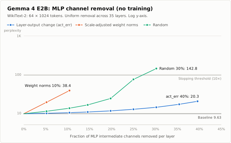
The graph is the experiment’s SVG with translated labels. The horizontal axis is nominal per-layer intermediate-channel removal, and the vertical axis is logarithmic perplexity. A line ending means evaluation ended there, rather than performance remaining constant afterward.
| Nominal removal | Base retained width | Double retained width | Parameters | act_err | Random | Adjusted norms |
|---|---|---|---|---|---|---|
| 0% | 6144 | 12288 | 4.63B | 9.63 | 9.63 | 9.63 |
| 5% | 5824 | 11648 | 4.55B (−1.8%) | 9.89 (1.03×) | 11.16 (1.16×) | 19.15 (1.99×) |
| 10% | 5504 | 11008 | 4.47B (−3.5%) | 10.27 (1.07×) | 13.42 (1.39×) | 38.42 (3.99×) |
| 15% | 5248 | 10496 | 4.40B (−4.9%) | 10.69 (1.11×) | 16.32 (1.70×) | — |
| 20% | 4928 | 9856 | 4.32B (−6.7%) | 11.44 (1.19×) | 23.99 (2.49×) | — |
| 25% | 4608 | 9216 | 4.24B (−8.4%) | 12.56 (1.30×) | 74.81 (7.77×) | — |
| 30% | 4288 | 8576 | 4.16B (−10.2%) | 14.18 (1.47×) | 142.8 (14.8×) | — |
| 35% | 3968 | 7936 | 4.08B (−11.9%) | 16.91 (1.76×) | — | — |
| 40% | 3712 | 7424 | 4.01B (−13.3%) | 20.27 (2.11×) | — | — |
Parameter counts cover the entire loaded text model, including untouched embeddings and attention. That is why model-wide parameter reduction differs from intermediate-width reduction.
Activation-Based and Random Selection
act_err reaches approximately 1.03 times baseline at 5%, 1.07 times at 10%, 1.19 times at 20%, and 2.11 times at 40%. Quality does deteriorate, but gently at small removal levels and more substantially with stronger removal.
Random selection reaches 1.16 times already at 5% and 1.39 times at 10%. It then reaches 2.49 times at 20%, 7.77 times at 25%, and 14.8 times at 30%, crossing the stopping threshold.
Identical retained widths can therefore produce substantially different prediction loss. Selection matters here as it did previously, but the useful criterion changed: individual magnitude worked for individual weights, whereas observed layer-output change worked for channels.
Where Norm-Based Selection Failed
The main evaluation’s adjusted-norm results are 19.15 at 5% and 38.42 at 10%, both worse than random selection’s 11.16 and 13.42. A deliberately designed importance score need not outperform no score.
Raw norms were not evaluated on the first 64 main-test windows. Adjusted norms at 15% and above were also unevaluated. The method-selection value of 439.4 cannot be inserted as a main-test result, and those missing conditions cannot be described as evaluated failures beyond the stopping threshold.
Adjusted norms at 10% reach approximately four times baseline, still below the ten-times threshold. That line ends because additional controls were not completed after evaluation slowed following model saving, rather than because the threshold was reached.
Scope of Statistical Comparisons
The experiment reports significantly better results for act_err than random selection at every shared stage from 5% through 30%, using paired-bootstrap 95% confidence intervals over 64 windows.
Pairing retains the difference in loss on the same text window. It helps separate method differences from variation in which windows are difficult. The question is whether the observed method difference is stable across this window set.
Those intervals do not establish the same difference for every newly drawn mask: only one random seed was used. They also do not include variability from retraining, other languages, or other corpora.
The summarized report supplies the significance conclusion, but not each interval’s endpoints or detailed statistical output. This article does not yet provide window-level raw data at the same granularity as the previous article’s JSONL. That difference in available evidence matters.
Comparison with Previous Unstructured Pruning
Matching Removed Weight Counts
The previous target set contained 205 attention and MLP matrices; this experiment removes MLP channels only. “10%” on their respective axes does not mean equal numbers of removed weights. Directly comparing those labels would confound selection with different removal budgets.
I therefore compared each channel-removal stage with the previous per-matrix unstructured method at the same removed-weight count. The previous experiment measured only five-percentage-point steps, so the comparison column is interpolated from those points, not newly measured at each matching fraction.
| Nominal channel removal | Measured act_err perplexity | Interpolated unstructured perplexity at equal removed-weight count |
|---|---|---|
| 0% | 9.63 | 9.63 |
| 5% | 9.89 (1.03×) | 9.63 (1.00×) |
| 10% | 10.27 (1.07×) | 9.72 (1.01×) |
| 15% | 10.69 (1.11×) | 9.89 (1.03×) |
| 20% | 11.44 (1.19×) | 10.33 (1.07×) |
| 25% | 12.56 (1.30×) | 11.22 (1.17×) |
| 30% | 14.18 (1.47×) | 13.37 (1.39×) |
| 35% | 16.91 (1.76×) | 21.27 (2.21×) |
| 40% | 20.27 (2.11×) | 45.50 (4.73×) |
At small removal budgets, selecting individual weights causes less degradation. Equal to the 10% channel stage, the unstructured interpolation is about 1.01 times baseline, versus 1.07 times here. Group removal imposes stronger constraints and less selection freedom.
Interpreting the Reversal at Larger Budgets
The ordering reverses at the 35% and 40% stages: 16.91 versus 21.27, and 20.27 versus 45.50. Under this weight-count mapping and interpolation, unstructured pruning is not uniformly better.
This is not a strict ranking of the methods. One column is measured and the other interpolated; target scope, selection criteria, and calibration data also differ. act_err uses text to estimate importance, while the previous magnitude method does not.
Where a curve changes sharply, interpolation cannot locate its crossing precisely. Saying that the table reverses at 35% does not identify an exact 35% threshold. Direct remeasurement of unstructured pruning at matching budgets would strengthen the comparison.
Prediction Quality and Implementation Benefits
Better unstructured perplexity at small budgets does not itself shrink arrays. Channel removal accepts somewhat larger prediction loss in exchange for smaller dense matrices, motivating the saved-model comparison.
Sparse storage and execution might also give unstructured pruning practical benefits. That was not tested here. The distinction is that the previous zeroing-only implementation did not obtain such benefits, rather than unstructured pruning being inherently incapable of acceleration.
Prediction retained per removed-weight budget and speed on the available runtime are separate axes. Both require measurement.
Saved-Model Selection and Quantization
Why Save the 10% Stage?
I saved the largest evaluated stage whose perplexity degradation stayed within 10%. The act_err 10% stage is about 1.07 times baseline, while 15% is about 1.11 times, so 10% met the chosen constraint.
This is not a proof of optimality. I did not search finely between 10% and 15%, the widths are constrained to multiples of 64, and other domains may not satisfy the same quality threshold.
The main evaluation series also informed this final stage selection. The first 64 test windows therefore participate in selecting the saved configuration. Saved-model perplexity is useful evidence, but is not an entirely new final test independent of all model selection.
Four Compared Configurations
The comparison covers original bf16, 10%-stage bf16, original 8-bit, and 10%-stage 8-bit. Quantization uses mlx-lm with group size 64, applied under the same settings to original and reduced models.
Channel removal reduces element count; quantization reduces representation size per weight. They can be combined. Because quantization alone changes capacity substantially, the extra removal benefit must be assessed between models with matching quantization.
| Metric | Original bf16 | 10% removal bf16 | Original 8-bit | 10% removal 8-bit |
|---|---|---|---|---|
| Parameters | 4.629B | 4.466B | 4.629B | 4.466B |
| Weight size | 9.26GB | 8.93GB | 4.92GB | 4.75GB |
| Peak MLX memory during generation | 9.61GB | 9.31GB | 5.47GB | 5.29GB |
| Prompt processing | 1,533 tokens/s | 1,637 tokens/s | 1,687 tokens/s | 1,794 tokens/s |
| Generation | 16.5 tokens/s | 17.5 tokens/s | 29.5 tokens/s | 32.7 tokens/s |
| Perplexity | 9.628 | 10.267 | 9.629 | 10.263 |
Quantization does not change parameter count. Its byte reduction reflects numerical representation. Channel removal does reduce count, from 4.629B to 4.466B. Keeping counts and bytes separate avoids treating all forms of “smaller” as equivalent.
Ten Percent of MLP Channels Is About 3.5% of the Model
At the saved stage, bf16 weights shrink by about 0.33GB and parameters by about 0.163B. The model-wide reduction is about 3.5%, quite different from nominal 10% channel removal.
The removable MLP weights constitute only about 34% of this model’s parameters. Much of the remainder is per-layer embedding tables and embeddings, untouched here. Looking only at the MLP removal fraction overestimates total effect.
For intuition, reducing a component that is 34% of the whole by 10% yields roughly 3.4% overall. The actual aligned 10% stage removes about 10.42%, consistent with approximately 3.5% overall. This is an explanatory estimate, not a substitute for counted saved parameters.
Even at the 40% stage, total parameters go from about 4.63B to 4.01B, approximately 13.3% reduction, while perplexity reaches 2.11 times baseline. Aggressive MLP-only removal leaves large untouched components while imposing increasing quality costs.
Quantization and the Additional Removal Benefit
Quantizing the original alone reduces 9.26GB to 4.92GB, close to half. Two bytes for bf16 versus one byte for 8-bit suggests a factor of two, but accompanying data means actual size is not exactly halved.
Perplexity changes only from 9.628 to 9.629 in this evaluation. Compared with channel removal, the capacity benefit is larger and the measured prediction change smaller. Generation also rose from 16.5 to 29.5 tokens/s, approximately 1.8 times. For reducing size in this environment, quantization was the more effective first operation.
Combining the two reduces 8-bit weights further from 4.92GB to 4.75GB, about 0.17GB, and generation peak memory from 5.47GB to 5.29GB. Quantization does not eliminate the additional benefit of smaller matrices.
I do not interpret 10.263 for the reduced 8-bit model versus 10.267 for reduced bf16 as a quality improvement caused by quantization. The difference is small and no statistical judgment for that difference is presented. The dominant removal degradation remains around 1.07 times, with a small additional quantization difference in this table.
Inference Speed and Memory
Benchmark Conditions
The prompt length was fixed at 512 tokens and generation at 256 tokens. Decoding was greedy and did not terminate on EOS, avoiding differences in output length caused by earlier stopping.
There were two launches with three runs each, six measurements total, summarized by their median. These are not single best-run values or timings for unequal output lengths. The records report non-overlapping generation-speed ranges between original and reduced models.
The six individual values and range endpoints are not included in the summary available here. I cannot derive new speed confidence intervals or claim identical percentage improvements in every run. The evidence is repeated observation of faster generation under the fixed-length condition.
Prompt Processing and Generation
For bf16, prompt processing improves from 1,533 to 1,637 tokens/s, about 6.7%, and generation from 16.5 to 17.5, about 6.3%. For 8-bit, the corresponding improvements are 1,687 to 1,794, about 6.3%, and 29.5 to 32.7, about 10.7%.
Processing input together and generating one token at a time have different computational shapes, so their speeds are recorded separately. This experiment does not isolate particular kernels or transfers, and prompt-processing results cannot stand in for generation measurements.
Reducing weights by 3.5% does not require time to fall by exactly 3.5%. Untouched computations, matrix widths, and quantization affect runtime. The observed improvement is not a proportional law guaranteed for other execution systems.
Improvement in Absolute Time
Using the displayed rounded throughputs for illustration, generating 256 tokens takes approximately 15.5 seconds for original bf16 and 14.6 seconds after removal. For 8-bit, the corresponding estimates are 8.7 and 7.8 seconds.
These are calculations from the table, not separate end-to-end measurements. They exclude model loading, calibration, input preparation, prompt processing, and UI overhead. They are not times from first launch to a completed answer.
They do indicate that the reported percentage improvements correspond to just under a second in the generation portion of this condition. Repeated use can accumulate savings, but quality cost and preparation expense must also be considered.
Peak-Memory Comparison
Generation peak memory falls by about 0.30GB for bf16, from 9.61 to 9.31GB, and about 0.18GB for 8-bit, from 5.47 to 5.29GB. It moves in a similar direction to weight size but is not identical to weight bytes.
Generation also needs caches and temporary buffers. These peaks apply to the fixed prompt and output lengths. Longer contexts can change the fraction occupied by untouched attention caches, so the short-condition reduction cannot be applied directly to long-context total memory.
A few hundred megabytes can matter on a 16GB machine. This reduction alone, however, does not make a model far beyond available memory suddenly fit. Quantization provided the larger effect in this experiment.
Changes in Generated Content
Quality Beyond Perplexity
In one same-prompt comparison, the original continued by correctly repeating a fact present in the prompt: a “Craig” role in 2004. The reduced model instead invented a role name and episode names.
This is one observed example, not a statistical error-rate study. It does not establish that the original is always correct or that the reduced model always fails. It does show why a roughly 7% perplexity increase is insufficient evidence for an interchangeable model.
The full prompt and continuations are not included in the records attached to this article. I do not fabricate quotations for a side-by-side example. I report only the observed difference and the single-example scope.
Small Average Differences and Application Requirements
Perplexity averages many next-token predictions. It does not replace evaluations of exact information extraction, conversational consistency, or executable code. A small mean difference can coexist with a large change on particular inputs.
Conversely, one failure does not establish unusability for every application. Application-specific testing with enough inputs is needed. This experiment establishes trade-offs in size, speed, and observed quality, rather than an adoption decision.
The within-10%-perplexity criterion was a threshold chosen for this experiment. For an application requiring reliable factual extraction, satisfying that threshold alone cannot establish acceptable behavior.
Environmental Changes and Unevaluated Conditions
Slower Evaluation After Saving
After saving the model, evaluation became approximately eight times slower than usual. Spotlight indexing was using roughly 85% CPU, and swap increased. Those observations suggest a cause, but I did not perform a controlled comparison changing only indexing activity.
This contributed to not evaluating raw norms on the main windows or adjusted norms at 15% and above. Missing conditions are not filled with failed or infinite values. Poor method-selection performance differs from measuring a main-test result.
It would also be incorrect to interpret the slowdown as the reduced model becoming eight times slower. The speed table is a repeated fixed-condition generation comparison; the slowdown is an environmental observation during additional perplexity evaluation.
Calibration–Evaluation Distribution Differences
Activation-based importance depends on calibration text. A channel quiet on WikiText-2 training data might matter for another language, code, or unusual symbol sequences. The test text comes from the same dataset, limiting generalization claims.
I did not test whether 64 calibration windows suffice, whether different windows select similar channels, or whether more calibration improves results. Activation-based selection outperforming norms does not establish optimal calibration.
Although method-selection windows differ from the main windows, the final removal stage was chosen using the main series. Evaluating the fixed saved configuration on new data would strengthen evidence for generalization.
Interpretation
Assessment of Weight-Based Importance
The first hypothesis was not supported by the selection rule tested. Adjusted norms at the 10% stage reached 3.99 times baseline perplexity, versus 1.39 times for random removal.
One possible reason is that ignoring normalization scales and input distribution disconnects raw magnitude from actual contribution. The large benefit of scale adjustment is consistent with that interpretation, but does not fully establish a cause.
Even adjusted norms being worse than random suggests that weight-only scores may rank actively useful channels too low. This is an interpretation of the outcome; the available records do not contain a complete correlation study between every channel’s score and output contribution. Identifying the responsible channels remains future work.
The difference from the previous experiment does not imply that magnitude is universally meaningless. Selecting individual elements and selecting entire gated nonlinear channels impose different constraints.
Assessment of Activation-Based Importance
The second direction was supported in these comparisons. act and act_err substantially outperformed norms during method selection, and main-test act_err outperformed random selection throughout the shared evaluated range.
This support applies to this model, calibration set, removal method, and evaluation range. It does not establish a universal activation score for all structured pruning. Small local output changes from single-channel removal also do not guarantee stable long generation after removal across many layers.
The progression from a failed convenient score to a criterion closer to the desired behavior was useful. Matching retained widths made it possible to compare how much prediction quality improved when the importance measure changed.
Scope of Actual Reduction and Acceleration
The saved 10%-stage model has fewer parameters and smaller matrices, lower generation peak memory, and higher measured throughput. This goes beyond the previous zeroing-only implementation to physical shape reduction.
The gain remains modest: weights shrink about 3.5% overall, bf16 generation improves about 6.3%, and perplexity worsens around 1.07 times, with an undesirable change in the generation example. Size, speed, and quality did not all improve simultaneously.
Quantization nearly halves weight size with little perplexity change on these windows. For reducing size in this environment, it had the larger benefit. Channel removal looks more like an additional adjustment alongside quantization than a replacement for it.
Reproducibility and Further Evaluation
Evidence Available with This Article
This article organizes tables and a graph from my experiment report. Authorship of the experiment does not mean that writing the article included another independent full execution. The code is in the experiment project’s experiments/gemma4_e2b_mlp_channels, separate from the previous gemma4_e2b_pruning experiment.
The machine-readable tables transcribe the rounded report values rather than raw measurements. The published evidence here is aggregated. It does not include individual timing runs, window-level NLL, importance arrays, retained masks, or saved-model hashes. The previous article’s raw data cannot regenerate this experiment’s intervals or saved model.
I distinguish structure checked in the versioned MLP implementation, outcomes recorded in the report, and interpretations. I do not invent executable reproduction commands for unshared implementation details.
Information Needed for Reproduction
Further documentation should fix the model revision, dependency versions, calibration-text selection, importance aggregation, and retained channels in every layer. The name act_err alone does not specify what is normalized, where output differences are measured, or which inputs are averaged.
For speed, retaining six individual measurements grouped by launch, loading and warmup treatment, execution order, cache settings, and memory state would make comparison on another day or machine easier. This improves reproducibility without invalidating the aggregate observations.
Generation examples should preserve the exact prompt and both continuations under matching conditions. One example cannot establish how frequently factual errors increase; more inputs are required.
Additional Conditions to Investigate
I would first vary both random masks and calibration-window selection to measure stability. This helps distinguish method differences from the particular text or mask chosen.
I would then relax uniform layer-wise removal and investigate allocation of a fixed reduction budget across layers. Aligned widths simplify loading, but layers need not tolerate equal fractions. Variable widths require considering implementation and storage as well as quality.
Quality evaluation should extend beyond WikiText-2 to other text, extraction, code, and long contexts. A single next-token metric cannot establish application suitability. Image and audio behavior remains outside the saved text-model evaluation.
Fine-tuning after removal is another question, but would be a different experiment from the no-training condition here. It would require recording training data and cost, recovered quality, and resulting speed and size together.
Conclusion
I saved and compared physically smaller Gemma 4 E2B models by removing MLP channels. Weight-norm selection failed, while act_err, calibrated using layer-output changes, worked better. At the nominal 10% stage, total weight size fell about 3.5%, generation throughput improved about 6.3% for bf16 and 10.7% for 8-bit, and perplexity deteriorated to about 1.07 times baseline.
Eight-bit quantization had the larger effect on size. It can be combined with channel removal, but the reduced model also showed a factual error in a generation example. Smaller storage, faster computation, and application-level interchangeability need separate verification.
The previous experiment asked which weights could be zeroed while preserving predictions. This one reached smaller executable matrix shapes on my runtime. The reduction was not dramatic, but selection changed quality substantially and produced measurable size and speed differences. Next I want to evaluate those quality changes over a broader range of inputs.