Reading The Lottery Ticket Hypothesis made me wonder how much of a large neural network could be removed while leaving something useful. I tried pruning Gemma 4 E2B, which fits on my Mac.
The short version: removing the smallest-magnitude weights separately in each target matrix increased perplexity by about 1.13 times at 20% pruning. Beyond that, degradation became steep: about 2.19 times at 30%, and 29.3 times at 40%. Random pruning reached about 13.4 times at just 10%. Which weights remain makes a substantial difference.
I did not retrain the model. This is an experiment with pruning a trained model, inspired by the paper, rather than a reproduction of the lottery ticket hypothesis.
Overview of the Lottery Ticket Hypothesis
This section explains Frankle and Carbin’s original paper. The later Gemma 4 E2B pruning experiment is a separate local investigation prompted by reading it.
The starting point is Jonathan Frankle and Michael Carbin’s “The Lottery Ticket Hypothesis: Finding Sparse, Trainable Neural Networks,” published at ICLR 2019. I use v5, dated March 4, 2019. Section, figure, and appendix numbers below refer to that version. Drawing on my reading notes, I want to explain enough of the paper to make clear what the experiment later in this article does and does not test.
Background of the Original Paper: Model Compression and Trainability
Pruning removes some of a trained neural network’s weights. For example, setting a connection between layers to zero prevents information from passing through that connection. If the neurons remain but their connections become scattered, the network becomes sparse.
If a large model can lose apparently unnecessary connections while retaining performance, it seems reasonable to build that smaller structure from the beginning. Then there would be no need for the original large model. We would like smaller networks to save training costs as well as storage and inference costs. That simple question motivates the paper.
But being reducible at the end of training differs from being trainable while small from the start. Perhaps training the large model was necessary to discover which connections to keep. Perhaps the surviving numerical values contain information acquired during training. Rebuilding the same small structure does not guarantee that it will learn in the same way.
The distinction is between the size needed to represent a final answer and the size that makes it easier to learn that answer. A small model might suffice for the first purpose while a larger one helps with the second. The lottery ticket hypothesis approaches this gap through initialization and subnetworks.
An analogy would be keeping only the route you walked on a map after finishing a hike, versus starting the hike knowing only that narrow route. This is an explanatory analogy, rather than a claim that optimization literally selects a single path. A small final structure does not establish that the process used to reach it was unnecessary.
Definition of a Winning Ticket
A winning ticket in this paper is not simply a small piece of a trained model with its learned weights intact. It combines a subset of the connections present in the original large network with the initial, pre-training values assigned to those connections.
Let θ₀ denote the original initialization and m a mask specifying which connections survive. Each mask entry is zero or one: zero disables a weight and one retains it. The smaller network’s initialization is then m ⊙ θ₀, where ⊙ means elementwise multiplication. The mask determines the connectivity; the initialization determines the starting values.
Training this part independently must reach test accuracy at least as high as the original with no more iterations, while using far fewer weights. A small model merely managing to learn something is not enough: size, accuracy, and training iterations are evaluated together.
In the definition in Section 1, let j be the iteration where the original network reaches minimum validation loss and a its test accuracy there. For the subnetwork, write these as j′ and a′. The requirements are j′ ≤ j and a′ ≥ a, with substantially fewer surviving weights.
The lottery metaphor can suggest that a correct answer is already encoded in the initial weights. But the network does not classify correctly without training. It still has to learn; the ticket wins through a starting point that makes effective learning possible.
Existence also differs from knowing the mask before training. The method trains the large network once and uses the outcome to discover a ticket. It is not an algorithm that identifies the right mask simply by inspecting initialization.
Training, Pruning, and Resetting to Initialization
The central procedure has four operations: randomly initialize a large network and save its initial values; train it; prune connections with small trained magnitudes; then restore the surviving connections to their saved original initial values.
Magnitude matters because the selection ignores sign. Between -0.8 and 0.01, the latter is closer to zero. Small magnitude is not necessarily a perfect measure of importance for every model. Here, it is a simple selection rule used to investigate how the resulting subnetworks learn.
The weights used to select the mask and the weights used to start the next training run come from different moments. Selection uses trained values. Retraining the sparse network does not carry those trained values forward: it restores the pre-training value at each surviving position.
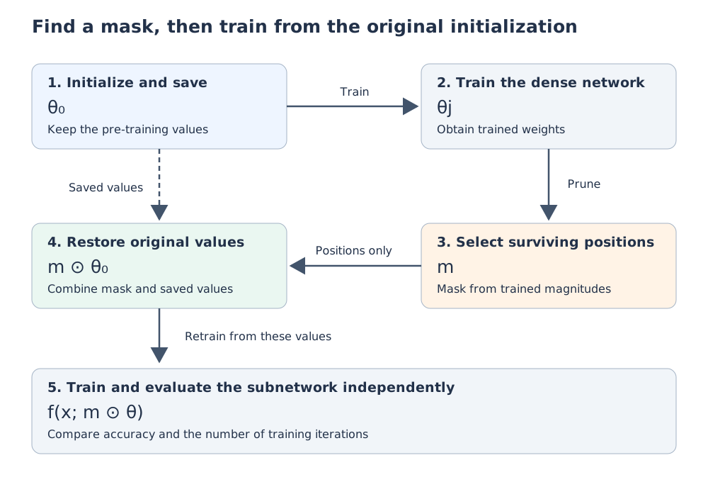
Keeping the trained values and fine-tuning would test how acquired values can recover performance. Resetting instead helps distinguish the benefit of carrying learned values forward from the benefit of the structure–initialization pair. This is precisely where my Gemma experiment differs.
One-Shot and Iterative Pruning
One-shot pruning trains once, removes the desired fraction of weights together, and resets the survivors. Iterative pruning, the paper’s main approach, repeats training, pruning, and resetting over multiple rounds. Each round selects additional removals from the connections that survived the previous round.
For an illustrative uniform rule that removes 20% of surviving weights each round, the remaining fractions would be 80%, 64%, and 51.2% after the first three rounds. This does not subtract twenty percentage points of the original total each time. The sequence is 0.8ⁿ. Actual experiments use different rates for some layers, including the output layer, so whole-network fractions need not follow that sequence exactly.
The paper finds that this gradual process can uncover smaller winning tickets than one-shot pruning. Learning again within an already narrowed network and selecting survivors from there works better than choosing all removals at once.
Appendix B also compares resetting after every round with continuing from learned values while pruning and resetting only once at the end. Both eventually test training from the original initialization, but they discover the mask through different paths. On Lenet and the Conv networks, resetting every round preserves accuracy and fast learning down to smaller sizes.
The final fraction of surviving weights is therefore not enough to describe the experiment. The training path used to find the mask also matters. Repeated training makes discovery expensive, however. The cost of training a known ticket once must be distinguished from the cost of finding it.
Control Experiments: Random Sparsity and Random Reinitialization
When reading this paper, it helps to separate two meanings of “random.” One control chooses the surviving connection positions randomly. Another keeps the mask discovered by pruning but draws fresh random initial values for the retained positions.
In the second case, the connectivity matches the winning ticket. What changes is whether each position uses its original value or a newly sampled one. A performance difference in that comparison cannot be explained by structure alone. It supplies evidence that pairing the structure with its original initialization matters.
That does not establish that structure is irrelevant. The mask was selected using training results, and at moderate pruning levels fresh initialization sometimes preserves accuracy. Structure and initialization both remain candidates; their effects can vary with pruning strength and training conditions.
The random method in my later experiment instead sets randomly selected weights of an already trained model to zero. Both the timing and the object being changed differ from the paper’s random reinitialization. Sharing the word “random” does not make those experiments equivalent.
Evaluation of Learning Speed and Accuracy
In the first part of the paper, the iteration of minimum validation loss is a proxy for learning speed. Validation loss measures prediction error on data not used for training. Continued training can keep fitting the training set while validation loss begins increasing again. The experiment asks how quickly the model reaches that minimum.
The paper calls this the early-stopping point and also measures test accuracy there. Appendix C explains the evaluation. A smaller model reducing training loss faster does not by itself show that test accuracy is preserved. Both speed and accuracy must be checked.
The early-stopping point is not an instruction to end the training used for pruning at that moment. For example, each Lenet round trains for a fixed 50,000 iterations. The recorded validation losses identify the minimum afterward. It is important to keep that measurement separate from the trained weights used to choose the pruning mask.
Fewer iterations also do not imply an equal reduction in elapsed time. If sparse weights are still processed in ordinary dense arrays, removing parameters may leave much of the computation per iteration unchanged. A claim such as “38% earlier” requires checking which count was reduced.
The main curves average multiple trials, and their error bars use minima and maxima. Those are neither confidence intervals nor records of just the best run. Reinitialization introduces additional random draws. This differs from the window-level bootstrap later in this article, starting with what variability is being measured.
Fully Connected Network Experiments on MNIST
The Lenet in Section 2 is Lenet-300-100, a fully connected classifier for MNIST handwritten digits. It is not the convolutional LeNet-5 that the name might suggest. It has hidden layers of 300 and 100 units followed by ten output classes.
The experiment prunes separately within layers based on trained weight magnitudes. The basic rate removes 20% per round, while connections to the outputs are pruned at half that rate. It uses Gaussian Glorot initialization, Adam in the basic setup, and 50,000 training iterations. It tracks how the training curves change as fewer weights survive while keeping the input and output task fixed.
The remaining-weight fraction is written Pₘ. This can be confusing: Pₘ = 20% means 20% remains, or 80% was removed. My later graph uses the removed fraction on its horizontal axis, so its direction is reversed.
The interesting Lenet result is that removing weights does not simply make everything worse. During the first pruning rounds, fewer surviving weights accompany faster learning and higher test accuracy. Further pruning eventually slows learning again and reduces accuracy. The original large model is not simply an upper bound from which performance declines monotonically.
The paper’s text reports that early stopping occurs 38% earlier with approximately 21% of weights remaining, and that a ticket with roughly 3.6% remaining returns to performance comparable to the original. I treat 38% as a number reported by the text. The reading notes identify a discrepancy with the mean curve in Figure 4, so I do not claim to have independently recovered that exact value from the figure.
It would be too strong to conclude that 96% of the original network is always unnecessary. The small structure was discovered using training of the original network and tested with the original initialization. The finding holds under the experiment’s data, optimization, and iteration budget. Removing weights does not make the discovery process disappear.
Evaluation of Optimization and Generalization
If a small model achieves higher test accuracy at early stopping but also higher training accuracy, optimization may simply have progressed faster. The paper therefore also compares models after the fixed training budget.
For Lenet, sparse networks can outperform the original on test data even where many conditions reach 100% training accuracy. They fit the training data equally well by that metric but behave differently on unseen examples. That supports the discussion of improved generalization.
I found this separation useful. Reducing loss faster, achieving better accuracy within a fixed training budget, and obtaining better test accuracy at matching training accuracy are different observations. Calling all of them “better performance” conceals which property changed.
This does not mean that smaller networks always generalize better. Excessive pruning reduces accuracy. There is a useful region between reducing a network with spare capacity and removing necessary representational capacity. Whether the same region exists for other data and models requires another experiment.
Convolutional Network Experiments on CIFAR10
Section 3 uses Conv-2, Conv-4, and Conv-6, reduced VGG-style networks for CIFAR10. A module contains two convolutional layers followed by pooling; the three networks have one, two, and three such modules, followed by fully connected layers.
Their weights are distributed differently between convolutional and fully connected layers. The paper consequently uses different pruning rates for those groups rather than imposing one universal rate. For example, Conv-2 and Conv-4 use basic per-round rates of 10% for convolutional weights and 20% for fully connected weights. Output connections use a lower rate again.
The broad pattern resembles Lenet. Iterative pruning produces a region with higher accuracy and fewer iterations to early stopping, followed by deterioration under stronger pruning. Keeping the mask but drawing new initial values causes performance to collapse sooner than preserving the original initialization.
However, randomly reinitialized Conv-2 and Conv-4 can retain or initially improve accuracy at moderate pruning levels. Initialization alone does not determine everything. It is reasonable to read this as evidence that the discovered structure itself may also have a useful bias for learning.
Winning tickets are also found with dropout. Dropout temporarily changes which units participate during training, whereas pruning permanently removes connections with a fixed mask. They are not interchangeable simply because both disable part of a network. Improvements when the two are combined provide evidence for thinking about how they interact.
Effects of Learning Rate and Warmup in Deep Networks
Section 4 studies CIFAR10 versions of VGG-19 and Resnet-18. Batch normalization, weight decay, data augmentation, and scheduled learning-rate reductions bring the setup closer to practical training. This Resnet-18 is a CIFAR10 architecture and should not be confused with the commonly used ImageNet model of the same name.
Applying the pruning procedure is no longer enough by itself. At high learning rates, some conditions produce similar performance with original and newly sampled initializations, failing to identify winning tickets. A favorable initialization does not work under every training configuration.
Lower learning rates make the advantage of restoring the original initialization easier to see. But the sparse models may then fail to reach the accuracy of the original network trained at a higher learning rate. Beating the reinitialized version of the same small network differs from matching the original large network. The former alone does not satisfy the winning-ticket criterion.
The paper therefore tests linear warmup: instead of using the target learning rate immediately, it increases gradually from zero. For VGG-19, a schedule rising to 0.1 over 10,000 iterations yields tickets that exceed the original accuracy down to 1.5% of weights remaining. Resnet also uses warmup, with different settings.
Changing the opening phase of optimization can change whether training succeeds with a given mask–initialization pair. I found that particularly interesting. The existence of a ticket differs from whether a chosen procedure can train it. Failure to find one depends on the search and optimization conditions.
For these deeper models, scheduled learning-rate drops also strongly influence accuracy curves, making a single early-stopping iteration a difficult speed comparison. The paper instead presents accuracy at several points during training. This explains why the presentation of evaluation changes between the earlier and later experiments.
Comparison of Layer-Wise and Global Pruning
For deeper networks, the selection scope changes too. Layer-wise pruning removes the same fraction separately in each layer. Global pruning pools the target convolutional layers and removes the smallest magnitudes across that pool. Appendix I.1 finds smaller winning tickets with the global approach.
Uniform layer-wise pruning assigns every layer the same fractional budget. Layers differ in size and role, so a small layer might become constrained early. Global pruning can retain more of one layer and remove more of another. It has a different degree of freedom.
In the Gemma experiment later in this article, per-matrix pruning performed better than global pruning. That does not refute the paper. Its image-classification experiments retrain from initialization after pruning, whereas mine evaluates a trained text-prediction model without retraining. The models and procedures differ, so the question of which selection rule preserves performance differs too.
Analysis of Initialization Properties
Appendix F examines winning-ticket initializations and connections. Its experiments address questions such as whether selecting large initial magnitudes is enough, or whether imitating the distribution of surviving initial values reproduces the benefit.
Pruning by initial magnitude before training performs worse than reinitializing a mask discovered through training. Sampling new values from the observed distribution of winning-ticket initializations also fails to reproduce their performance. Matching each layer’s histogram is not a sufficient explanation.
Interestingly, the surviving weights are not necessarily those that moved least during training. The appendix instead examines a tendency for them to move farther and increase in magnitude. A good initialization might sound like one already close to its final correct value, but that explanation is insufficient.
Experiments also add noise to the initial values. Small changes do not destroy everything, although larger noise hurts performance. Initialization mattering does not mean that every bit must remain identical. This makes a winning ticket seem different from simple memorization of a lucky numerical pattern.
The discussion points toward combinations of structure, initialization, optimizer, and data. The paper does not complete a theory explaining why those initial values work. I read these experiments as narrowing possible explanations by investigating observed differences.
Winning-Ticket Existence and the Conjectured Behavior of SGD
The experiments investigate whether a large network contains a small subnetwork capable of learning. The paper also goes further with a conjecture: perhaps ordinary SGD itself searches for and trains a favorably initialized subnetwork.
These claims should be kept separate. Showing that a part extracted afterward can learn independently does not immediately establish that training the original dense model was a process of selecting that part. Weights removed later might have affected gradients and representations along the way.
The idea that larger networks contain more candidate combinations is intuitive. But the number of candidates does not explain why a particular optimizer reaches a good one. The paper treats that extension as an untested conjecture.
I want to distinguish what made the paper interesting to read from what its experiments establish. The idea that a large model contains a small useful part caught my attention. Rephrasing it as “learning merely picks up an answer already present” would go beyond the evidence.
Constraints on Model Reduction and Computational Savings
Section 6 on limitations identifies the focus on MNIST and CIFAR10 image classification, the repeated training required for discovery, and the fact that the resulting sparse structures were not directly optimized for the hardware of the time.
Unstructured pruning removes scattered matrix entries. Even with logically fewer active weights, array dimensions remain unchanged. Without implementations that skip zeros or formats that efficiently store values and their positions, actual memory use and runtime may not fall as much as expected. The implementation considerations differ from structured methods that remove whole channels or blocks.
If finding a small model takes fifteen or more training runs, faster training of that model may still cost more overall for a single use. Its practical value depends on whether the mask can be reused, whether discovery can finish earlier, and whether it can transfer to other tasks.
Even so, I found the paper interesting as a way to separate ease of learning from the size of the final representation. Beyond compressing a model by discarding unnecessary weights, it asks why beginning with a large model helps. It uses a method for making models smaller to investigate why large models can learn.
Research Significance and Potential Applications
At this point, a reasonable question is: if discovering the small model takes repeated training, what is the benefit? That bothered me too. Some benefits are already visible in the paper’s experiments; others are applications that the findings might eventually enable. Drawing on the application prospects in Section 1 and the discussion in Section 5, this is how I understand them.
Independent Trainability of Sparse Subnetworks
The experiments first show that reaching accuracy comparable to a large network does not necessarily require updating all its connections throughout training. A discovered winning ticket can learn independently and match the original. In some ranges, accuracy improves and the required iteration count falls.
When we want a large model’s accuracy, matching its parameter count is not the only possibility to investigate. Selecting connections and starting values that learn effectively becomes another option. This does not mean that any connections or values will work. Replacing the model with a smaller one without investigating that selection can fail, which is precisely why discovering trainable combinations matters.
This goes beyond observing that removing weights from a finished model leaves its outputs intact. The surviving part can do more than store a learned answer: with its original starting values, it can learn again. The useful prospect is treating the small structure as a unit of training, rather than only as a compressed finished product.
Potential Training-Cost Savings from Early Discovery
The clearest practical hope is training cost. If a good mask could be found early and the remaining work performed in a small network, we might avoid running the large network through the entire process. The paper identifies searching and pruning as early as possible as a future direction.
However, running its iterative pruning procedure does not establish lower total training cost. Discovery requires repeated training. Showing that a small part can learn differs from developing a cheap way to find it. The latter is needed before claiming an overall saving.
For illustration, let discovery cost be S, the cost of training the original model once be D, and the cost of training the ticket once be T. If we assume the same ticket can be used N times under the same conditions, the comparison is N × D against S + N × T. Even if T < D, a single use might not recover the discovery cost.
This equation is an explanatory accounting example, rather than a measurement from the paper. Cheap sparse execution and ticket reuse each need separate validation. Transfer to another task is not guaranteed either. Still, it makes the possible improvements concrete: earlier discovery, reuse, and faster sparse operations.
Implications for Architecture and Initialization Design
When designing a smaller model, reducing depth or width is an obvious starting point. These experiments suggest examining both which connections exist and the values from which they learn. Reinitializing an unchanged mask can alter the result, so copying connectivity alone is insufficient.
If recurring connectivity patterns or initialization properties of winning tickets became understood, they could guide the design of small structures and initializations that learn effectively from the beginning. That is the direction behind the paper’s proposed application to better network design. Studying those properties does not mean a general design method is already available.
For my own small-model experiments, this also means that poor accuracy need not immediately be attributed only to too few weights. I can separately investigate connection selection, its pairing with initialization, and learning-rate conditions. Together with the warmup results, the paper provides useful controls for diagnosing failures.
Analysis of Model Capacity and Generalization
The paper finds ranges in which pruning improves test accuracy over the original. That is a benefit visible in the experiments. Making a model smaller need not always be framed as sacrificing a little accuracy to save resources. Under some conditions, smaller and more accurate coexist.
Excessive pruning still hurts. Comparing different test accuracies at matching training accuracy helps investigate which structures generalize beyond the training examples, rather than only which ones fit those examples easily. Pruning becomes an experimental intervention for exploring capacity and generalization.
This does not guarantee that pruning my LLM will make it smarter. The paper’s image classification and my text prediction have different conditions. The useful outcome is not a universal rule that pruning improves performance; it is a way to ask comparable questions about what to retain, how much to remove, and how to train what remains.
Implications for Overparameterization and Optimization
Conceptually, the findings separate the capacity needed to represent a final prediction from the conditions needed to reach it through learning. A model being reducible after training does not show that starting large served no purpose. Conversely, a small discovered part learning independently indicates that factors beyond size help make learning possible.
This leads to questions about how excess parameters assist optimization and how initialization affects the learning trajectory. The conjecture that SGD searches for a favorable part is one possible explanation. It is not a completed answer, but the experiments let us investigate structure and initialization within the same model by holding one fixed and changing the other, rather than treating large and small models as unrelated objects.
My main takeaway was that I no longer had to view weights as a uniform block. A model trained using all its weights can contain combinations that learn independently. That makes me want to modify the weights and investigate which combinations survive and under what conditions they remain useful.
The Gemma pruning experiment is an entry point to that interest. Modest degradation after removing 20% does not establish reduced training cost or discovery of a winning ticket. It first examines selection rules that preserve trained predictions, leading to further questions about retraining, sparse implementations, and performance on other data.
Purpose and Scope of the Gemma Pruning Experiment
Returning to what I can do on my Mac, I have Gemma’s pretrained weights rather than its initialization before pretraining. I am not repeatedly reproducing the original training either. I therefore cannot test learning from the same initialization, which is central to the hypothesis.
Instead, I check how much prediction performance remains immediately after connections are removed from the trained weights. I compare removing small magnitudes per matrix, removing them globally, and removing weights randomly. These conditions reveal differences between masks, but not between initializations.
The metrics differ too. The paper measures image classification accuracy; my perplexity measures next-token prediction in text. Rather than comparing the numbers directly, I borrow its approach of fixing some factors and changing others to identify differences.
With that distinction in place, modest degradation after removing roughly 20% of target weights does not mean I have found a winning ticket. A large gap between random removal and magnitude-based removal does show that the choice of surviving connections matters in the trained model under this evaluation. That is the narrower, measurable question I chose to pursue on my own machine.
Experimental Environment and Pruning Targets
I used the pretrained base model google/gemma-4-E2B, with bf16 weights. The snapshot was 433813a669639fd7eaa83155828e9000ed357d53. The environment was an Apple M3 Mac with 16GB RAM, Python 3.13.17, MLX 0.32.4, mlx-lm 0.32.2, NumPy 2.5.5, and PyArrow 26.0.1.
The pruning targets were attention q/k/v/o and MLP gate/up/down weight matrices in the 35 decoder layers: 205 matrices containing 1,835,532,288 weights. The last 20 layers share KV and have no k/v matrices of their own. Embeddings, per-layer embedding (PLE) tables and gates, norms, and the output head were excluded.
“20% pruned” below means 20% of these target weights, rather than 20% of the whole model.
I compared three methods:
| Method | Selection |
|---|---|
Per matrix (layerwise) | Remove the same fraction of smallest-magnitude weights from each matrix |
| Global | Pool all 205 matrices and remove the smallest-magnitude weights |
| Random | Select each weight independently with the same probability in every matrix |
Here, layerwise operates on individual weight matrices, rather than treating a decoder layer as one group. Random pruning selects elements probabilistically, so its count is not exact.
For magnitude pruning, the implementation builds a histogram of bf16 magnitude bit patterns to locate a threshold for the requested count. Ties at the boundary are resolved using random numbers. Pruning proceeds cumulatively as sparsity increases, keeping previously removed weights at zero. The original model is reloaded between methods. Only one random seed, 0, was used.
Evaluation Data and Metrics
The evaluation used the WikiText-2 raw test split. Text was concatenated and tokenized, then the first 64 windows were selected. Each window contains BOS followed by 1,023 text tokens, for a total length of 1,024. There are 65,472 predicted tokens in total. Every condition uses the same windows.
The metric is next-token perplexity, where lower is better. It is the exponential of mean negative log-likelihood (NLL); doubling perplexity does not mean halving accuracy.
I increased pruning in five-percentage-point steps and stopped evaluating a method once its perplexity exceeded ten times the unpruned baseline. There was no fine-tuning or reset to the original initialization.
Evaluation-Window Construction and Loss Calculation
Even on WikiText-2, segmentation changes perplexity. I joined the Parquet text column with two newlines and tokenized it with add_special_tokens=False. The log records 292,282 tokens, yielding 285 windows of 1,023 text tokens. Only the first 64 windows were evaluated, rather than the entire test split.
Each window receives one leading BOS token. The model receives all but the final token, and the sequence shifted by one position supplies the targets. Loss is evaluated for all 1,023 text tokens. Context does not carry between windows: each begins again with BOS. The values should therefore not be compared directly with benchmarks using different context lengths or overlapping windows.
For each position, the loss is logsumexp(logits) - target-token logit. Summing this over all 65,472 predicted tokens and dividing by that count gives mean NLL. The table’s perplexity is exp(mean NLL), rather than the arithmetic mean of 64 window perplexities.
The model computes bf16 logits, and conversion to float32 for loss calculation is divided into chunks of 256 positions. This avoids making one enormous float32 copy without removing prediction targets. Mean NLL for each window is also recorded to five decimal places; those records are used for confidence intervals.
Pruning-Mask Generation
Magnitude-based pruning constructs a histogram from bf16 bit patterns with the sign bit cleared. There are 32,768 possible codes, so a threshold can be found by counting entries rather than sorting all weights as floating-point values.
The target count is round(pruning fraction × element count) for each matrix in layerwise, and for all target matrices together in global. Entries below the threshold are removed, and random values break ties at the threshold. The implementation intends to match the target count, but does not include an index-based fallback for collisions in the random tie-break values.
The random method selects each entry when its uniform random value is below the requested fraction. Reusing the same random key for each matrix at successive levels makes the masks nested: an entry removed at 5% stays removed at 10%. Magnitude-based pruning also proceeds cumulatively with previously zeroed weights retained.
To the six decimal places stored in the results, actual zero fractions match the requested values except at random 10%, recorded as 0.100007, or approximately 10.0007%. These measured fractions are included in results.jsonl.
Relationship Between Pruning Fraction and Perplexity
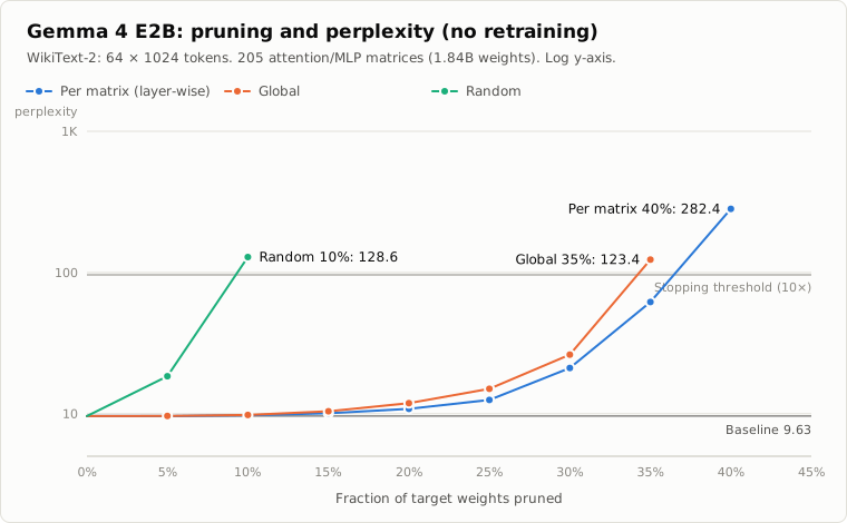
The graph is an SVG generated from the experiment’s results JSONL, with its labels translated into English. Its “layer-wise” method operates per weight matrix, as described here.
Parentheses show the ratio to the unpruned baseline. Dashes indicate conditions that were not evaluated after stopping.
| Fraction of target weights pruned | Per matrix | Global | Random |
|---|---|---|---|
| 0% | 9.63 | 9.63 | 9.63 |
| 5% | 9.63 (1.00×) | 9.65 (1.00×) | 18.44 (1.92×) |
| 10% | 9.74 (1.01×) | 9.80 (1.02×) | 128.6 (13.4×) |
| 15% | 10.06 (1.05×) | 10.41 (1.08×) | — |
| 20% | 10.84 (1.13×) | 11.89 (1.23×) | — |
| 25% | 12.53 (1.30×) | 15.00 (1.56×) | — |
| 30% | 21.06 (2.19×) | 26.21 (2.72×) | — |
| 35% | 61.77 (6.42×) | 123.4 (12.8×) | — |
| 40% | 282.4 (29.3×) | — | — |
At 5% per-matrix pruning, perplexity rounds to the same 9.63 as the baseline. A paired bootstrap over windows with 10,000 resamples gives a mean NLL difference of approximately +0.0002 and a 95% confidence interval of approximately [-0.0005, +0.0009]. No difference was detected within this evaluation set. That does not prove identical performance.
The model initially tolerates pruning surprisingly well: 1.01 times baseline perplexity at 10%, and 1.13 times at 20%. But degradation rises rapidly beyond roughly 30%. Random pruning already reaches 1.92 times at 5% and 13.4 times at 10%. Simply choosing small-magnitude weights makes a large difference.
Global pruning performed worse than per-matrix pruning at every shared evaluation level from 5% through 35%. The 95% confidence intervals for their differences in recorded per-window NLL are above zero at each level. At 5%, the mean NLL difference is approximately +0.0020, with an interval of [+0.0013, +0.0026].
For magnitude-based pruning, the implementation finds a shared threshold in the global case. I have not investigated which matrices account for the degradation.
Detailed Perplexity Values and Evaluation Stopping Criteria
The per-matrix 5% result rounds to the same 9.63 as the baseline, but their unrounded values differ. For stopping, the baseline’s unrounded value defines the threshold of ten times baseline perplexity.
Per-matrix pruning goes from 61.7703 at 35% to 282.4349 at 40%, stopping after the 40% result. Global pruning goes from 26.2099 at 30% to 123.3804 at 35%, stopping at 35%. Random pruning goes from 18.4391 at 5% to 128.5886 at 10%, stopping at 10%.
These are the first sampled levels exceeding the threshold, rather than a continuous search for its exact crossing. Global pruning being below the threshold at 30% and above it at 35% does not establish an exact collapse point of 35%.
Confidence-Interval Estimation and Interpretation
The comparison uses a paired bootstrap retaining correspondence between the same 64 windows. For each window, I subtract the reference condition’s mean NLL from the pruning condition’s mean NLL, giving 64 differences. I sample those differences with replacement and take their mean 10,000 times. The 2.5th and 97.5th percentiles form the 95% confidence interval. The summary seed is 1, distinct from the pruning seed of 0.
For comparisons against the original model, a positive difference means deterioration. Subtracting per-matrix NLL from global NLL likewise makes positive values indicate worse global performance. These intervals do not describe variability over model training or multiple pruning seeds. No adjustment is made for simultaneously comparing several pruning fractions.
An interval containing zero does not prove the absence of a difference. It means that this data and evaluation did not distinguish a very small difference. It does not establish that 5% removal is harmless for every input.
Memory-Use Mitigation and Changes to Execution Conditions
The production results came from three executions with interruptions and resumes, rather than one continuous run.
Swap slowed down the first run, which I stopped during the 20% per-matrix evaluation. I then limited MLX caching and split the conversion of logits to float32 into chunks before resuming. After the model degraded substantially at 40%, I added the stopping rule and interrupted the 50% evaluation. The third execution completed the remaining methods.
Recorded MLX peak memory fell from 11.25GB before the changes to 10.5GB afterward. Evaluations in the third execution took approximately 123–126 seconds per condition, excluding pruning and model loading. The first baseline evaluation took 576.6 seconds. Because execution conditions changed, these timings do not provide an inference-speed comparison between models. Memory headroom mattered on a 16GB Mac.
Mapping Executions to Result Records
The first execution finished loading the model at 15:45:30. It recorded the baseline and per-matrix 5%, 10%, and 15%, then stopped during the 20% evaluation. These are rows 1–4 of the result file. Model acquisition was approximately 9.6GB and took 465 seconds according to the execution records.
The second execution finished loading at 16:16:43 and used --resume. It skipped evaluation of the four existing conditions, but replayed pruning from the original model to reach 20%. It recorded five conditions from 20% through 40%, then stopped during the 50% evaluation. These are rows 5–9.
The third execution finished loading at 16:37:54. It reconstructed the masks again, recognized that the recorded per-matrix 40% result exceeded the ten-times-baseline threshold, and skipped higher levels. It then recorded seven global conditions and two random conditions, finishing at 16:59:15. These are rows 10–18.
The incomplete 20% and 50% evaluations are not filled in as successful results. The first, second, and third execution logs are available to follow the sequence. Progress-bar lines are omitted from the logs.
NLL, Evaluation Time, and Memory Use Across All 18 Conditions
The following table is generated from the result file. Every condition, including the baseline, evaluates the same 64 windows and 65,472 prediction targets. Time is eval_s; memory is MLX’s peak_gb, rather than process RSS or total OS memory use. The recorded peak is the value reported at that point, not an incremental allocation attributable solely to that condition.
| Method | Pruned | Mean NLL | Evaluation (s) | MLX peak (GB) |
|---|---|---|---|---|
| Baseline | 0% | 2.264722 | 576.6 | 11.25 |
| Per matrix | 5% | 2.264925 | 230.9 | 11.25 |
| Per matrix | 10% | 2.276571 | 299.1 | 11.25 |
| Per matrix | 15% | 2.308953 | 386.4 | 11.25 |
| Per matrix | 20% | 2.382841 | 142.5 | 10.50 |
| Per matrix | 25% | 2.527897 | 162.7 | 10.50 |
| Per matrix | 30% | 3.047452 | 255.9 | 10.50 |
| Per matrix | 35% | 4.123422 | 283.3 | 10.50 |
| Per matrix | 40% | 5.643448 | 217.4 | 10.50 |
| Global | 5% | 2.266877 | 126.1 | 10.50 |
| Global | 10% | 2.282618 | 122.7 | 10.50 |
| Global | 15% | 2.342991 | 122.6 | 10.50 |
| Global | 20% | 2.475500 | 122.9 | 10.50 |
| Global | 25% | 2.708196 | 122.7 | 10.50 |
| Global | 30% | 3.266138 | 122.5 | 10.50 |
| Global | 35% | 4.815272 | 122.8 | 10.50 |
| Random | 5% | 2.914472 | 125.0 | 10.50 |
| Random | 10% | 4.856618 | 123.0 | 10.50 |
The logs record approximately 1.8 seconds for random pruning itself and 9.7–10.7 seconds for global pruning. Those times are excluded from the evaluation column. These records do not establish that higher pruning fractions always evaluate faster: swap and implementation changes affect the timings, and execution was not converted to sparse operations.
Two-Window Smoke Evaluations and Numerical Consistency
Before the production evaluation, a short run compared the baseline with per-matrix 50%. Another smoke run tried 5%, 10%, 20%, 30%, and 40%, showing modest changes at lower levels and a sharp collapse around 30–40%.
| Per-matrix pruning fraction | Perplexity on two windows |
|---|---|
| 0% | 7.635695 |
| 5% | 7.624526 |
| 10% | 7.704467 |
| 20% | 8.413256 |
| 30% | 15.921080 |
| 40% | 325.312759 |
| 50% | 168,754.311435 |
This combines multiple smoke-result files, whose evaluation range differs from the production table’s 64 windows. A slightly better value at 5% on just two windows does not justify a performance-improvement claim.
After the memory changes, repeating the same two conditions produced 7.6356949852 for the baseline and 168754.3114353944 for per-matrix 50%. The earlier baseline was 7.6356952130: there is a tiny numerical difference, but it does not change the table’s interpretation. This smoke check confirmed similar values with chunked loss calculation; it was not an independent reproduction of every production condition.
Experiment Code, Result Data, and Reproduction Procedure
The pruning and evaluation code, summary script, synthetic-data tests, and 18-row results JSONL are available. The original chart generator reads the same results file.
The tests check pruning counts, magnitude ordering, a shared global threshold, and nested random masks. The comparison between cumulative and direct pruning requires mask agreement greater than 0.999, rather than exact equality. While preparing this article, I checked the NLL, perplexity, and token counts in all 18 records and independently checked the rounded confidence interval at 5% pruning.
The model snapshot must be fixed to reproduce the original weights. The supplied evaluation script otherwise loads the model by name. Its --resume checks do not establish complete input identity, so reuse an output file only when the evaluation conditions match.
python3.13 -m venv .venv
.venv/bin/pip install mlx==0.32.4 mlx-lm==0.32.2 numpy==2.5.5 pyarrow==26.0.1
mkdir -p data results
curl -L -o data/test.parquet \
  https://huggingface.co/datasets/Salesforce/wikitext/resolve/main/wikitext-2-raw-v1/test-00000-of-00001.parquet
.venv/bin/python test_prune.py
.venv/bin/python prune_ppl.py --model /path/to/fixed-model-snapshot \
  --data data/test.parquet --out results/results.jsonl \
  --windows 64 --methods layerwise,global,random \
  --sparsities 0.05,0.1,0.15,0.2,0.25,0.3,0.35,0.4,0.5,0.7,0.9 \
  --stop-ratio 10
.venv/bin/python summarize.py results/results.jsonl
Scope and Limitations of the Experimental Results
For this text-prediction evaluation, pretrained Gemma 4 E2B tolerated setting a modest fraction of its small-magnitude target weights to zero. The evaluation covers only the first 64 WikiText-2 windows, with no tests of conversation or code generation. Confidence intervals describe this window set, rather than variability across models or random seeds.
The weight arrays retain their original shapes. I did not change storage or computation to use sparse representations, so this experiment does not demonstrate smaller model files, lower memory use from pruning, or faster inference.
Fine-tuning might allow more pruning, but I have not tested that. Resetting to the original initialization and training, as required to test the lottery ticket hypothesis, also remains outside this experiment. For now, it was interesting to see the gentle change up to around 20% and the steep collapse beyond it, just by removing weights on my own machine.